Celebrating 20 Years of H.264: the foundation of modern Internet Streaming

Exactly 20 years ago, May 2003, the Joint Video Team (VCEG and MPEG) approved the first version of the video codec known as H.264/AVC, a groundbreaking standard that would forever change the world of video. H.264, not only revolutionized video compression but also gave birth to and propelled the era of Internet streaming. It has enabled billions of computer, mobile devices, tv sets to record and playback videos with increasing capabilities over the years, adapting to the progressive increase of connections speed and video resolutions. It has democratized video creation and consumption and has been crucial in making video ubiquitous.
Today, H.264 stands as one of the most successful international standards in the history of computer science, and its resilience over time demonstrate the exceptional work done by those brilliant researchers and scientists 20 years ago.

Standards play a crucial role in ensuring interoperability and preventing the concentration of technology control. H.264’s success as an open standard has empowered a diverse range of manufacturers, content creators, and streaming platforms to embrace and adopt it. This has fueled innovation, competition, and collaboration, benefiting end-users with a rich multimedia experience across devices and applications.

I like to mention also two other key events that have helped H.264 to become the de-facto standard for video streaming: the debut of an efficient H.264 decoder in the Flash Player (2007 – Flash Player 9) and the birth of the OSS encoder x264 (2004). The first event empowered almost 1 billion desktop computer with the capability to decode H264 videos inside a browser, without switching to an external application. Several years later H264 was adopted by every browsers natively with HTML5 Video but in those early years H264 in Flash Player enabled / enhanced the experience provided by foundational services like Youtube or BBC’s iPlayer.

The second mentioned event is not less important. x264 has contributed to an efficient implementation of H.264 encoding. The work started by Laurent Aimar and masterfully continued by, among the others, Loren Merritt and Fiona Glaser, has been truly exceptional and foundational as well.

Looking ahead, the question arises: can future codecs seamlessly carry the torch from H.264 and guide us through the next 20 years with the same virtuosity? The technology landscape is constantly evolving, and advancements are being made in video encoding and streaming. Subsequent codecs, such as H.265 (HEVC) and the more recent AV1 and VVC, have emerged, promising improved compression efficiency and enhanced visual quality.

Furthermore, future-generation codecs aim to address the growing demand for higher resolutions, immersive experiences, and bandwidth optimization. They will leverage cutting-edge techniques, including machine learning and artificial intelligence, to further refine video compression algorithms. However, they will face the challenge of not only surpassing H.264’s technical capabilities, which after 20 years is an easy task, but also gaining widespread adoption and compatibility across a vast ecosystem of devices and platforms. A real challenge indeed: earning the trust, the enthusiam of the entire video ecosystem, that enthusiasm that made H264 so crucial and so obiquitous to our industry.

As we celebrate the 20th anniversary of the standardization of H.264, let us acknowledge its immense contributions to the world of video and thanks to everyone who contributed to this revolution. Happy birthday H264.

FCS and RTMP – Streaming Technologies from the future

I remember clearly the enthusiasm and excitement when I moved my first steps in streaming and real-time communication. I was already fond of video compression and interactive web and was working actively with Flash community to create interactive experiences, but my career took a turn when Macromedia released Flash Communication Server 1.0. It was September 2002 and after 20 years the RTMP protocol, one of its foundational technology, is still among us!.

Pritham Shetty (helped by Jonathan Gay – the father of Flash) was the ingenious main author of this milestone in the history of video streaming. Pritham had already an extensive expertise in real-time communication for the web and for example, in 1996 he developed for NTT a Java based web client for connecting multiple users in a synchronized experience. And again, in 1996 a personalization server he developed was used even by Netflix! (when it was still very distant from the company we use to know today).

FCS was an exceptional server capable to enable real-time communication, live and on-demand video streaming features in Flash Player 6.0. The architecture of FCS was really ahead of its time and when I started working with it I had only a 640Kbps down/128Kbps up ADSL connection and a 64Kbps GPRS phone and nonetheless it was possibile to communicate in real time with other users over such connections and create futuristic interactive applications.

As we all know, 18 years after this exceptional release, the entire world has depended on real-time communication technologies like Microsoft Teams, Google Meet or Zoom because of Covid-19 pandemic. Think of FMS as a playground where Flash developers could easily develop video conference applications similar to those, with multiple audio-video-data streams produced in the browser by Flash, transported via RTMP protocol, orchestrated server-side by FMS and consumed again on a Flash Client.

I think the main advantage of this stack was simplicity and elegance and I’ve always used the lesson learned with FCS in my career as an Architect of Media Solutions. At the FCS’s foundation there was a non-blocking I/O stack scriptable in Action Script 1.0 (essentially JavaScript). Every user connection, application startup, disconnection and in general interaction raised an event and the code responded with actions or async I/O operations to connect RTMP streams in publish mode to RTMP stream in subscription mode and orchestrate via script many other interactions and data sharing (Curiously the architecture is very similar to Node.js. When Flash was abandoned I started easily to work with an early Node and FFmpeg to substitute many of the use cases I used to serve with FCS).

The simplicity and high efficiency of RTMP is also the main reason why it is still used today. RTMP allows to stream interleaved audio, video and data tag on TCP, SSL or tunneled in HTTP(S) and it’s possible trasparently to pass from real-time (few ms), to live and to vod use cases, with RPC call interleaved in the stream and easily recordable for interactive reproduction of communication’s sessions.


When working with this stack you had literally infinite possibilities a decade before webRTC was conceived and I ended to be an expert in FCS (then known also as Flash Media Server / Adobe Media Server) developing many advanced applications in the next 10 years (for example, thanks to the flexibility of the duo Flash + FCS I was able to design one of the first implementation of adaptive bitrate streaming for the first catch-up TV in Italy in 2008). 

Unfortunately FCS/FMS/AMS has not had the success and the widespread diffusion it deserved because of an absurd and limiting pricing model by Adobe. Nonetheless it has left an undeniable contribution to the Internet streaming.

Happy 20th Birthday RTMP and kudos to the great FCS and its authors.

Defeat Banding – Part II

Recently Banding has finally become an hot topic in encoding optimization. As discussed in this previous post, it is nowadays one of the worst enemy for an encoding expert especially when trying to fine-tune content-aware encoding techniques.

Banding emerges when compression reduces too much high frequencies locally on a frame and this splits a gradient in individual bands of flat colors. Those bands are therefore easily visible and reduce the perceptual quality.

For years I’ve underlined that even a useful metric like VMAF was not able to efficiently identify banding and that we needed something more specific or a metric like VMAF but more sensible to artifacts in dark or flat parts of pictures and hopefully a no-reference metric to be usable for source file assessment as well as compressed ones.

FIG.1 – Lack of correlation between VMAF and MOS in case of sequences with banding (Source: Netflix)

As anticipated in the previous post, I started in 2020 experimenting with some PoC about a metric to measure banding and the next year I validated the logic working for one of my clients at a “bandingIndex” metric. I’ll call it bIndex for sake of simplicity.

Significantly, even Netflix was working on banding and presented (Oct 2021) their banding detection metric Cambi. Cambi is a consistent no-reference banding detector based on pixel analysis and thresholding, plus many optimizations to have solid and accurate banding identification.

The logic I’ve used is very different from Cambi and can be used to identify not only banding but many types of impairments using what I call the “auto-similarity” principle.

The logic of source-impaired similarity

The logic I explored is illustrated in the picture below:

FIG 2 – Auto-Similarity principle

A source video is impaired to introduce an artifact like blocking, banding, ringing, excessive quantization and similar.

if the impaired version of a video is still similar to the not-impaired self, this means that the original video has already a certain degree of that impairment. That degree is inversely proportional to the similarity index.

I call it “source-impaired similarity” or sometimes “auto-similarity” because a video is compared to itself plus an injected, controlled and known impairment. The impairment need to be one-off and not cumulative. Let me explain better:

For one-off impairment I mean a modification that produces its effect only the first time it is applied. For example a color-to-gray filter has that characteristic, if you apply it a second time, the result doesn’t change anymore.

Now we have to things to choose: the impairing filter and the similarity metric.

So let suppose we want to find if a portion of video has banding, or excessive quantization artifacts, we can, in this case, use as impairment a quantization in frequency domain. This form of impairment has the characteristic described above: when applied multiple times, only the first application produce a distortion, the next ones do not modify the picture that’s already quantized with a known quantization level.

The most used similarity metric is SSIM. It maxes to 1 when videos are identical and goes below 1 when dissimilarities arise. It is more perceptual aware than PSNR and more insensible to small deltas as long as statistical indicators like mean, variance and covariance are similar.

It’s very important to analyze the video divided in small portions and not as a whole, especially during metric fine-tuning, to better understand how set thresholding and verify the correct identification of the artifact. Then it is possible to calculate also an “area coverage percentage” that provides interesting information about the amount of frame area impacted by the artifact under test (banding or other).

The high level schema below illustrates the metric calculation. The fine tuning of the metric requires other processings like pre-conditioning (that may be useful to exalt the artifact), appropriate elaboration of SSIM values to keep only the desired information (non-linear mapping and thresholding), final aggregation of data to summarize (pooling) a significative index for each frame.

FIG. 3 – Extraction of bIndex

Conclusions

To develop, verify and fine tune the bIndex metric, I extended a custom player I developed in the past for frame-by-frame and side-by-side comparison. In the pictures below you can see indexes for each frame-area that are green when banding is not visible and are red when banding is visible and annoying. The first picture shows also an overlayed, seekable timeline that plots the banding likeliness for each picture area and the threshold that differentiates between irrelevant and visible/annoying banding. In this way it’s possible to seek quickly to frame sequences that contain banding and evaluate the correctness of the detection.

This approach could be extended to many types of artifacts and used to assess various types of video (sources, mezzanines, compressed video) with different thresholds. Having statistical indicators from frame coverage percentage is also useful to take decisions like source rejection or content re-encoding with specific profiles to fix the problem. Note that currently the thresholds have been identified using perception of small panels of golden-eyes on big-screens but in the future more complex modeling could be used to correlate the objective numbers with perception and introduce other improvements like time-masking and context-aware banding estimation.

HYPER: a decade of challenges and achievements.

Who follows me since the years of Flash Player and Adobe Media Server knows that I’ve been busy in the last 15 years developing encoders, players and in general software architectures to enable, enhance and optimize video streaming at scale. I’ve achieved many professional successes working on innovative projects for companies like NTT Data, Sky, Intel Media, VEVO and many others. In such contexts I’ve had the opportunity to meet inspiring people: managers, engineers, colleagues and ultimately friends that helped me in growing as an engineer and as a video streaming architect.

In particular this 2021 I celebrate the 10th anniversary of Hyper, one of those achievements, but let’s start from the beginning:

Conception

In 2008 I started collaborating with Value Team, a leading system integrator in Italy (later acquired by the global innovator NTT Data). The BBC’s iPlayer was just released and media clients started asking for something similar, so NTT Data contacted me to design a high performance platform (encoder and player) for the nascent market of catch-up TVs and OTT services. The product, VTenc, powered the launch in 2009 of the first catch-up tv in Italy (La7.tv owned by Telecom Italia).

The most innovative feature of VTenc was the possibility to encode a single video in parallel, splitting it in segments then distributed on a computing grid for parallel encoding. The idea emerged after a discussion with Antony Rose and his team (the creators of BBC’s iPlayer) where they underlined that one of the main problems in encoding for a catchup tv was the long processing time that delayed the distribution of the encoded stream after the conclusion of the show on tv.

A few months and many technical challenges later, the feature was ready. And the idea of the parallel encoding was successfully applied to La7.tv: we received the live program in “parts”, emitted every time there was an advertisement slot. Each part, usually 20-25 min long, was diveded into smaller chunks, encoded in parallel and then reassembled and packetized with a map-reduce style paradigm. Also thanks to a client side playlist, the final result was ready for streaming after just 10 minutes from the conclusion of the live show.

An incredible result for that time because commercial encoders required many hours for an accurate 2-pass encoding of assets 2-3 hours long. It was also one of the first implementations in absolute for adaptive bitrate streaming in Flash (Custom implementation in Flash Player 9 + AMS when Adobe introduced officially adaptive bitrate only in Flash Player 10).

The birth of Hyper

VTenc was improved in the following years until in 2011 NTT Data signed a deal with Sky Italy to provide the encoder for the new incoming OTT services of the broadcaster.
We implemented new features and they choose VTenc for a variety of key points:

– flexible queue management system
– rapid customizability
– high video quality
– high density and scalability
– short time to market.

VTenc evolved into something more complex, NTT Data Hyper was born. The model was something different than buying a commercial encoder that usually had long evolution cycles and well defined but unflexible road maps. Hyper has been something more similar to a focused, tailor made and optimized encoding engine like those build by Netflix or Amazon. Often also a sandbox where to conceive and test new technologies and ideas.

In this 2021 we celebrate the first 10 years of Hyper.

A decade of innovative achievements and milestones

Since then we have reached many achievements and milestones facing the challenges of the last decade. Looking back, it has been an exciting journey, professionally intense and enriching. Some achievements that deserve to be mentioned:

– A long story of content-aware encoding approaches from the first empirical versions (2013) to the use of ML to implement peculiar “targetMOS” and “targetDevice” encoding modes (2017+). I’ve been always a fan of “contextual optimizations” and started my experiments in the years of Flash Video, presenting some initial ideas at Adobe Max 2009-11 but then I’ve had the opportunity to implement those paradigms in the industry in various “flavors”.

Internal caching logic for elementary streams that allows the quick repurposing of previously encoded assets without executing a new expensive encoding. With this logic we have been able many times to repurpose libraries (tens of thousands assets) in a matter of days. In this way, add a new audio format, change ident, parental or other elements in the content playlist, or add a new packetization format (es: new version of HLS) has been always quick and inexpensive.

– In 2016 Hyper evolved from a grid computing to a hybrid cloud paradigm with on-prem resources that cope with baseline workload and cloud resources that satisfy peaks. Having thought the software since the beginning around agnostic services and flexible work queues, the hybridization was a natural step. Resources can be partitioned to have maximum throughput and cost efficiency on some queues as well as minimum time-to-output on others. 

– In this last context my team designed a 2-step technique to generate on the fly a smart mezzanine with controlled perceptual quality to quickly and conveniently move very big high quality sources to the cloud for parallelized encoding (with a bandwidth reduction of up to an order of magnitude). 

– Full cloud deployments on AWS and GCloud that quickly and dynamically scale from just 2 on-demand instances to thousands spot instances (“elastic texture”) with optimized scaling logics to minimize infrastructure costs and provide higher reactivity than standard scaling systems like autoscaling groups.

Now that Hyper turned 10 and after various millions of encoding jobs, in 2021 we are going to finalize Hyper v2 and tackle new challenges (VVC, AV1, complete refactoring, perceptual-aware delivery, agnostic architecture to apply massively parallelized processing to other contexts), but that’s the matter for an entirely new story…by now let’s celebrate:

happy 10th birthday Hyper!  


15 years of blogging about Internet Video

15 years ago I started this blog to share my esperiments and points of view around video streaming, playback and encoding. It has provided important opportunities to my professional career and extended my circle of contacts in the world of video streaming professionals, and for that I’m grateful…

Unfortunately (or fortunately depending by the point of view) I’ve not always had the time a blog deserve, especially in the last 5 years… but after more than a hundred articles and almost 2 Million contacts I can say that the objective has been nevertheless achieved.

In the meanwhile the trends of technical communication changed profoundly, We’ve seen the rise and trasformation of social media platforms like Facebook and Twitter, the increasing role of Linkein in presenting and sharing Ideas in a professional environment or the role of Youtube as one-stop-shop for presentations and conferences. I think however that a blog can still be a useful place where to consolidate, share and persist ideas and contribute to the community.

For the future, I’m trying to reorganize my activities to find more spare time to disseminate knowledge and experiences had especially in the last 10 years, writing more posts and partecipating more to web conferences (hoping then to restart live partecipation asap).

It could be interesting to completely refresh my series FFmpeg-The Swiss Army Knife of Video Internet (there are so many things to say about it and ways to use it more productively) or analyze technically the state-of-the-art codecs like AV1 and VVC like I did for H.264 and H.265 in the past, or again continue to analyze optimization’s trend and new challenges, especially related to video processing architectures.

I’m rolling up my sleeves, stay tuned…

Defeat Banding – Part I

In my last post I have discussed about what I think to be the current arch-enemy of video encoding: “banding“.

Banding can be the consequence of quantization in various scenarios today, particularly when the source is a gradient or a low power textured area and your CAE (Content Aware Encoding) algorith is using an excessive QP.

Banding is more frequent in 8bit encoding but is possible also in 10bit encoding and is also frequent in high quality source files, or mezzanines when they have been subject to many encoding processes.

Modern block based codecs are all prone to banding. Indeed I find h265, VP9 and AV1 to be even more prone to banding than h264 because of wider block transforms (and that contributed to an increase of banding in Youtube and Netflix videos in recent times).

As discussed in the previous post, it is easy to incur in banding also because it is subtle and it’s not easy to measure it. Metrics like PSNR, SSIM but even VMAF are not sensible to banding even if it is easy for an average viewer to spot it, at least in optimal viewing condition.

This is an example of banding:

Picture with banding on the wall

The background shows a consistent amount of banding especially in motion, when the “edges” of the bands move coherently and form a perceptually significative and annoying pattern. Below the picture has the Gamma exalted to better show the banding.

Zoomed picture with exalted gamma

Seek to prevent

To prevent banding is first of all necessary to be able to identify it. This by itself is a complex problem.
Recently I’ve tried to find a way (there are many different approaches) to estimate the likeliness of having perceptually significative banding in a specific portion of a video.

I’m using an auto-correlation approach that is giving interesting preliminary results. So this “banding metric” analyzes only the final picture, without reference to source files (than, in case of mezzanine or sources you obviouly do not have anyway).

For example: here we have a short video sequence. When you watch at it in optimal viewing condition, you can spot some banding on flat areas. The content is quite dark (maybe you can spot someone of familiar in the background 😉 so, as usual, in the continuation I’ll show preferably the frames with exalted gamma.

The algorithm produces the following frame-by-frame report where an index of banding is expressed for each quadrant of the picture (Q1 = Top Left quadrant, Q2 = Top Right quadrant, Q3 = Bottom Left quadrant, Q4 = Bottom Right quadrant).

Below you can see the Frame 1 with exalted gamma. From the graph above, we see that the quadrant with higher banding likeliness is Q2. For the moment I’ve not yet calculated the most appropriate threashold for perceptually visible banding, but empirically it is near 0.98 (horizontal red line) . So in this frame, we have low likeliness to have banding and only a minor probability for Q2.

FRAME 1

In the frame below we have an incresing amount of banding, especially in Q1 but also in Q2 (on the tree and sky). The graph above shows an increasing probability of perceptually visible banding in quandrant Q1 and Q2 and infact they are above the threashold, while Q3 and Q4 are below.

FRAME 173

Then there’s a scene change, and for the new scene the graph reports an high probability of banding for quadrant Q1 and Q3 (click on the image below to zoom) an oscillating behaviour for Q2 (the hands are moving and the dark parts exibit banding in some parts of the scene) while the Q4 quadrant is completely immune from banding.

FRAME 225

Preliminary conclusions

Has discussed, it’s very important to start from the identification and the measurement of banding because if you can find it, you can correct encoding algorithms to better retain details and avoid introducing this annoying artifact. It’s also useful to analyze sources and reject them when any banding is found, otherwise any other consequent encoding will only worsen the problem. The journey to defeat banding is only at the beginning… wish me good luck 😉

Thoughts around VMAF, ContentAwareEncoding and no-ref metrics


Introduction

Content-Aware Encoding (CAE) and Context-Aware Delivery (CAD) represent the state-of-the-art in video streaming today, independently from the codec used. The industry has taken its time to metabolize these concepts but now they are definitely mainstream:

Every content is different and needs to be encoded differently. Contexts of viewing are different and need to be served differently. Optimization of a streaming service requires CAE and CAD strategies.

I’ve discussed several times these logics and the need for CAE and CAD strategies and I’ve implemented different optimizations for my clients during the years.

Speaking about Content-Aware Encoding, at the beginning we used empiric rules to determine a relationship between the characteristics of the source (eventually classified) and the encoding parameterization to achieve a satisfying level of quality at the minimum possible bitrate. The “quality metric” used to tune the algorithms was usually the compressionist’s perception (or that of a small team of Golden-Eyes) or more rarely a full-featured panel for subjective quality assessment. Following a classical optimization approach (read some thoughts here) we subdivided a complex “domain” like video streaming in subdomains, recursively trying to optimize them individually (and then jointly, if possible) and using human perception tests to guide the decisions.

More recently, the introduction of metrics with high correlation with Human Perception, like VMAF, have helped greatly in designing more accurate CAE models as well as in the verification of the actual quality delivered to clients. But, are all problems solved ? Can we now completely substitute expert’s eye and subjective tests with unexpensive and fast objective metrics correlated to human perception ? The answer is not simple. In my experience, yes & no. It depends on many factors and one of them is accuracy…


A matter of accuracy

In my career I’ve had the fortune and privilege to work with open-minded Managers, Executes and Partners who dared to exit their comfort zone to promote experiments, trials and bold ideas for the sake of quality, optimization and innovation. So in the last decade I’ve had the opportunity to work on a number of innovative and stimulating projects like:
various CAE deployments, studies on human perception to tune video encoding optimizations & filtering, definition of metrics similar to VMAF to train ML algorithms in most advanced CAE implementations and many others. In the continuation of the post I’d like to discuss some problems encountered in this never-ending pursuit for an optimal encoding pipeline.

When VMAF was released, back in 2016, I was intrigued and excited to use it to improve an existing CAE deployment for one of my main clients. If you can substitute an expensive and time consuming subjective panel with a scalable video quality tool, you can multiply the experiments around encoding optimization, video processing, new codecs or other creative ideas about video streaming. A repeatable quality measurement is also useful to “sell” a new idea, because you can demonstrate the benefits it can produce (especially if the metric is developed by Netflix and this brings immediate credit).

However since the beginning VMAF showed in my experiments some sub-optimal behaviors, at least in some scenarios. In particular, what I can even now recognize as the Achille’s heel for VMAF is the drop of accuracy in estimating perceptual quality in dark and/or flat scenes.

In CAE we try to use the minimum possible amount of bits to achieve a desired minimum level of quality. This incidentally brings to very low bitrates in low complexity, flat, scenes. On the other hand, any error in estimating the level of quantization, or target bitrate in such scenes may produce an important deterioration of quality, in particular may introduce a amount of “banding” artifact. Suddenly, a point of strength of CAE becomes a potential point of weakness because a standard CBR encoding could avoid banding in the same situation (nervertheless with a waste of bitrate).

Therefore, an accurate metric is necessary to cope with that problem. Banding is a plague for 8- bit AVC/HEVC encoding, but can appear also in 10-bit HEVC video, especially when the energy of the source is low (maybe because of multiple elaborations) and a wrong quantization level can completely eliminate higher, delicate, residual frequencies and cause banding.

If we use a metric like VMAF to tune a CAE algorithm we need to be careful in such situations and apply “margins” or re-train VMAF to increase the sensibility in such problematic cases (there are also other problematic cases like very grainy noise, but in those I see an underestimation of subjective quality, which is much less problematic to handle).

I’m in good company in saying that VMAF might be not the right choice for all scenarios because even YouTube in the Big Apple 2019 Conference pointed out that VMAF is often not able to recognize properly the presence of banding. 

youtube_band
Figure 1. VMAF overestimates quality on dark, flat, scenes

I could hypothesize that this behavior is probably due to the way quality has been assessed in VMAF, for example the distance of 2.5xH could reduce sensibility in those situations, but the problem is still present also in VMAF 4K where distance is 1.5xH so maybe is a weakness of the elementary metrics.


A case in 4K

Let’s analyze a specific case. Recently I’ve conducted a Subjective Quality test on 4K contents, both SDR and HDR/HLG. VMAF 4K is not tuned for HDR so I’ll limit my considerations to the SDR case. The subjective panel has been performed to tune a custom quality metric with support for HDR content that then has been used to train an ML-based CAE deployment for 4K SDR/HDR streaming.

The picture below shows a dark scene used in the panel. On the left you have the original source, on the right you have a strongly compressed version (click on picture to enlarge).

Figure 2. Source (left) vs Compressed (right). Click to Enlarge
Figure 3. Exalted gamma to show artifacts on encoded version. Click to Enlarge

In Figure 3 you can easily see that the image is very damaged. It’s full of banding and also motion (obviously not visible here) is affected, with “marmalade” artifact. However, VMAF reports an average score of 81.8 over 100, equivalent to 4 in 1to5 scale MOS, which overestimates the subjective quality.

The panel (globally 60 people, 9000+ scores , 1.5xH from 50” 4K display, DSIS methodology) reports a MOS of 3.2 which is still high in my opinion, while a small team of Golden EYE reported a more severe 2.3.

From our study, we find that variance in the opinion scores for such type of artifacts increases considerably, maybe because of different individual visual acuity and cultural aspects (not trained to recognize specific artifacts). But a Golden Eye recognizes immediately the poor quality and so also an important percentage of the audience (in our case 58% of the scores were 3 or below) will consider the quality not sufficient, especially for the expectation of 4K.

This is a classical problem of taking into consideration the mean when variance is high. VMAF provides also a Confidence Interval, that’s useful to take better decision but still the prediction has an overestimated “center” for the example above and at least 2 JND distant from the MeanOpinionScore (not to mention Golden Eye’s score).  

Anyway, below we can see the correlation between VMAF 4K and subjective evaluation in a subset of the SDR sequences. The points below the area delimited by red lines represent content in which the predicted quality is overestimated by VMAF. Any decision taken using such estimation may lead to a wrong decision and some sort of artefacts.

vmaf4k_scatterplot1
Figure 4. MOS vs VMAF 4K


Still a long journey ahead

VMAF is not a perfect tool, at least not yet. However, it has paved the way toward handy estimation of perceptual quality in a variety of scenarios. What we should do probably is to consider it for what it is: an important “step” in a still very long journey toward accurate and omni-comprehensive quality estimation.

For now, if VMAF is not accurate in your specific scenario, or if you need a different kind of sensitivity, you can re-train VMAF with other data,  change/integrate the elementary metrics or make your own metric that focuses on specific requirements (maybe less universal but more accurate in your specific scenario). You could also use an ensemble-like approach, mixing various estimators to mitigate the points of weakness.

I see also other open points to address in the future:
– better temporal masking
– different approach to pooling scores both in time and spatial domain
– extrapolation of quality in different viewing conditions

As a final consideration, I find YouTube’s approach very interesting. They are using no-reference metrics to estimate the quality of source and encoded videos. No-reference metrics are not bound to measure the perceptual degradation of a source-compressed couple of videos, but are designed to estimate the “absolute” quality of the compressed video alone, without access to the source.

I think they are not only interesting to estimate quality when the source is not accessible (or is costly to retrieve and use), like in monitoring of existing live services, but they will be useful also as internal metric for CAE algorithms.

In fact, modern encoding pipelines try often to trade fidelity to the source with “perceptual pleasantness” if this can save bandwidth. Using a no-reference metric instead of a full-reference metric could increase this behaviour similarly to what happened in super resolution passing from a more traditional cost function in DNN training to an “adversarial-style” cost function in GAN.

But this is another story…

Let’s rediscover the good old PSNR

In the last years, I’ve been involved in interesting projects around how to measure and/or estimate perceptual quality in video encoding. Measuring quality is by itself useful during encoding optimizations development and monitoring to assess the benefits of an optimized pipeline. But it’s even more interesting to estimate quality you can achieve with specific parameters before encoding so to be able to implement advanced logic in Content-Aware Encoding.

It’s a complex topic but I’d like to focus in this post on the role that PSNR can still have in measuring quality.

Is PSNR not much correlated to perception?

PSNR is well known to be not much correlated to perception. SSIM is a bit better but both show to be scarcely correlated from a general point of view, or at least so it seems:

PSNRvsMOS_0

The scatter-plot shows a number of samples encoded at different resolutions and levels of impairment and PSNR vs MOS (perceptual quality in standard TV-like viewing conditions). You can see that the relationship between PSNR and MOS is not very linear and for example a value of 40dB corresponds to MOS ranging from 1.5 to 5, depending on the content.

It is clear that we cannot use PSNR as an indicator of absolute quality in an encoding. Only at very high values, like 48dB the significance of the measure is useful.

It is because of that scarce correlation with MOS (the optimal metric would stay on the green line in the graph above) that Netflix has defined a metric like VMAF.

VMAF uses a different approach: it calculates multiple elementary metrics and using machine learning build a “blended” estimator that works much better than the individual elementary metrics.

I have worked on a different, but conceptually similar, perception-aware metric in the past. So I know that such metrics may have a problem: are a bit expensive to calculate. This is not because of ML that’s very fast when inferencing, but because you need to use accurate and slow elementary metrics (or a higher number of faster metrics) to have good results in the estimation.

Can PSNR still play a role?

In the common experience, PSNR still communicates something to the compressionists. Professionals like Jan Ozer continue to advocate PSNR for certain type of assessment and I agree that, for example, it is very appreciable especially in relative comparisons, probably thanks to its “linearity” inside specific testing frames. Knowing how ML based metrics work, I admit that PSNR is much more linear and monotonic “locally” while this is not guaranteed in case of ML-based estimators (it depends heavily on the ML-algorithm).

PSNR vs MOS

So, let’s take a look at this scatter plot. The cloud of points provides little information but if we connect the points related to the same video source we see that a structure starts to emerge.

The relationship between PSNR and MOS for the same source can be linearized in the most important part of the chart with an error that in some project can be negligible.

So what we are lacking to use PSNR as a perceptual quality estimator?

We need some other information extracted from the source that provides us with a starting point and a slope. With a fixed point on the chart (es: the PSNR needed to reach 4.5 MOS for a given source) and a slope (the angular coefficient of the approximated linearization of the PSNR-MOS relationship for that specific content), we could be able to use PSNR as an absolute perceptual quality estimator simply projecting the PSNR to the line and recovering the corresponding MOS.

PSNR vs MOS2

Now I’m experimenting exactly around how to quickly find a starting point and a slope from the characteristics of the specific source (scene by scene, of course). The objective is to find a quick method to estimate those params (point and slope) so to be able to measure absolute perceptual quality an order of magnitude quickly than with VMAF (probably with lower accuracy too, but still with good local linearity and monotonic behavior).

This may be very useful in advanced Content-Aware Encoding logic to measure/estimate the final MOS of the current encoding and, for example, adjust params to achieve the desired level (CAE in live encoding is the typical use case).


“Time Machine” – my talk at Demuxed 2018

I’ve just returned from a wonderful experience at Demuxed 2018.

speaker1I have had the honor to participate as a speaker alongside professionals from Twitter, Netflix, Youtube, Twitch, Comcast, Intel, Mux, Bitmovin, Akamai … and in general, the experience as both attendee and speaker has been amazing.

The event was streamed live on Twitch but today have been released also the individual VoD recordings (sessions list), including mine.

My session is:

“Time Machine” – how to reconstruct perceptually, during playback, part of the detail lost in encoding.

posterTM

In the last years, I’ve focused my efforts on “joint” optimization of various elements of the streaming pipeline. Evolving from an intra-domain to a inter-domains optimization approach, it is possible to squeeze out much more efficiency.

I’ve worked on joint optimizations of encoding and players, for example. Sometimes throwing in the mix also “augmentations” of protocols. If the player knows how the encoder is optimized it’s possible to develop improved heuristics and vice-versa with a synergic effect. I’ve already discussed a bit about that trend in this previous post.

In this scenario, I have discussed during Demuxed about another un-usual possibility of joint optimization:

Reconstruct perceptually part of the detail loss in encoding using in the Player a GPU-based reconstruction model that uses information extracted by the encoder or ML to estimate the best parameters.

It’s an old idea I’ve been insisting on for years as a way to ultra-optimize the streaming pipeline, with different tunings for high quality and high-efficiency cases (es: mobile).
I proposed a proof-of-concept based on Flash in a 2010 trilogy of posts and spoke about it also at Adobe Max 2010 in Los Angeles.

After the decline of Flash I’ve waited for WebGL to be more generally available in browsers and devices to make the idea evolve. Now WebGL is very powerfull and filtering with complex pixel shaders also high-resolution content is not a problem.

I’ll elaborate more on the logic in a future post. By now, take a look at the recorded speak and/or at PDF presentation: Presentation-Demuxed2018-FabioSonnati.

I’ve been very satisfied with the level and quality of feedbacks on the topic and in general Demuxed has been a wonderful occasion to meet and chat with high level professionals of the streaming business.

Artificial Intelligence in video encoding optimization

ai

Without doubt A.I. is the buzzword of the moment. We can definitely find it used everywhere, ranging from image classification/recognition to language translation, from sentiment analysis to market predictions, not to mention autonomous driving, fitness bands, latest CPUs/GPUs, smartphones and so on. A.I. prophets promise a new era of “intelligent” computing that will disrupt the way we live and use technology.

ML_trend
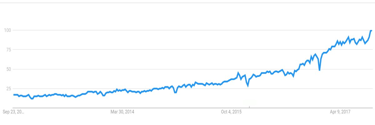
Fig1. Google Trend for “Artificial Intelligence”

Is it all that glorious? Even if all that glitters is not gold and many of the expectations are over inflated I think that A.I. (or it’s more correct to call it Machine Learning for most of the applications) is already truly capable to empower engineers with new tools and ways to solve problems, make accurate predictions and design complex systems.

As such, why don’t we apply it also in the field of encoding and streaming optimization?

but let’s start from the beginning…


Artificial Intelligence Machine Learning


From now on I’ll speak about Machine Learning and not Artificial Intelligence. AI is more a marketing slogan than an accurate term to depict current achievements (read this maybe oversimplified yet efficient comparison). In fact, many of the applications often branded as AI-driven are indeed more simply based on ML algorithms.
Not to mention that now that AI is at its peak of inflated expectations in the Gardner’s hype cycle, a lot of more traditional technologies are opportunely rebranded with the new, bold term just to exploit the wave.

ML is not indeed new. It is rooted in the late 50s and 60s when scientists started to study algorithms that can “learn” from data and make predictions based on that data. Algorithms capable to model complex systems from sample inputs and make data-driven predictions or classifications without active modeling by engineers.

ML is based on or is adjacent to other well know disciplines like computational statistic, mathematical optimization, operation research, linear programming; All popular university courses in not so ancient times.

ML has been widely used in the industry for years with success. Every time you use your credit card, a ML-based algorithm estimates the probability of a fraud thanks to classification algorithms trained on a huge amount of transactions (someone has said BigData?). Recognition of digits, OCR, speech recognition, spam detection are other consolidated applications. More recently you find ML-based algorithms in fitness bands to recognize/classify the activity done by users. Netflix has created a famous recommendation engine using ML. Google uses ML extensively for speech recognition, search ranking, form completion, translations. Apple uses it for Siri, among other things and any image classification application is based on deep learning and CNN that are at the cutting-edge of ML.

So it’s true that ML is powerful but it’s nothing exotic. It is essentially a discipline that provides algorithms, methods and best practices that help engineers in creating complex models without analyzing necessarily the underlying phenomena.

Indeed, modeling is something engineers already often do in their daily work. But sometimes analyze and modelize a complex phenomenon is not easy at all. I have already talked about optimization approaches and complex modeling in this post. At the end, instead of studying a complex system by inferring the rules of its subsystems (a classic way to proceed), ML provides engineers with a set of tools to create much more accurate models starting from a wide number of observations and data.

There are many algorithms, techniques, procedures and approaches in ML. A broad distinction is made between supervised learning, unsupervised learning and reinforcement learning. And inside supervised ML we can mention algorithms like linear regression/classification, Support Vector Machine, Random Forest, Decision Trees, Ensemble Methods, Gradient Boosting, Ada Boost and so on, and then continue with the Neural Networks family: Deeplearning, Convolutional NN, Recurrent NN, LSTM RNN, etc…

Wow, it’s a wide and complex landscape where it’s not simple and immediate the choice of the algorithms, the fit and the optimization of the entire system.

There are important points to considerate:

1. ML is a tool-set but then is up to the engineers how to use it in creative and efficient manner. ML doesn’t work by itself!

2. Many ML-algorithms behave like a black-box and it is not easy to extract knowledge of the underlying phenomena from that black-box. Sometimes is preferable a simpler algorithm than a more complex (and more efficient) one when you want to better comprehend the system under study.

3. Overfitting is everywhere! It’s the worst enemy and requires much attention especially to avoid creating models that in reality perform worse than empiric approximations.


Machine Learning as a tool to optimize video encoding 


In this post I compared optimization to function approximation/estimation. It’s easy to see the parallelism between function approximation and ML-based regression techniques. Using ML is possible to create a model that “predicts” with a good accuracy the behavior of a system for unknown inputs using only a number of known sample points to train/fit a chosen ML algorithm and minimize the associated cost function.

A mix of ML algorithms can be very useful everytime you have to “optimize” something.
Minimize a cost function means, in fact, optimize and we have already said that ML is based on mathematical optimization, operation research and linear programming, disciplines strictly correlated to the concept of “optimization”.

So even video encoding is a fertile field for ML-driven optimization. In video encoding, we have many independent variables (metrics that describe the features of the video, resolution, target quality, etc…) and the final objective could be (but not only) to minimize quality/bitrate ratio using the right encoding parameterizations.

In recent years Youtube and Netflix have used ML to achieve optimization of specific objectives in video encoding. In the case of Youtube, they have used NN to predict quantization levels that produce the desired target bitrate so to be able to obtain the performance of a dual pass encoding in a single pass. This is an example of optimization of the quality/speed ratio because in the Youtube’s scenario the huge amount of input videos determines a high cost of encoding that this approach tries to optimize.

Netflix has instead used ML (SVM in the specific case) to fuse the performance of elementary objective metrics in a unique reliable subjective quality estimation (VMAF metric, Video Multi-Method Assessment Fusion). VMAF has been used then as an enabling technology for other optimization processes.


Content-Aware to the next level: Perception-based encoding


In the last year, I’ve been involved in an extensive and on-going project of NTT Data that uses ML to optimize encoding. The objective of the project is to take Content-Aware encoding to the next level and be able to encode with a target perceptual quality on screens of different size. I already introduced this as a new emerging trend in a previous blog-post.

Instead of specifying a resolution and bitrate, like in a traditional encoding, now we can specify only the target perceptual quality (es: a MOS rate from 1 to 5) and the max size of the screen on which the video has to be watched. The ML-driven algorithm will determine the encoding parameterizations for each scene of the video to achieve the desired perceptual quality when watched on that target screen size. A high complexity scene will require a higher average bitrate while a low complexity scene will require a lower bitrate. But the actual value and many parameters will depend on input content metrics, target MOS and target screen size.

Such a level of optimization provides a way to minimize the bandwidth consumption using only the amount of bits necessary to achieve the desired level of quality across different screen sizes. At the same time, using advanced player’s heuristics is possible to exploit the VBR encoding produced in output to increase also the QoE during streaming, delivery in average an higher quality compared to traditional types of encoding (es: CBR o capped VBR with a target avg bitrate).

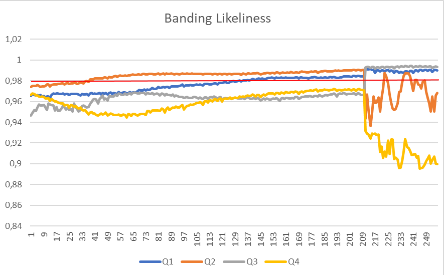
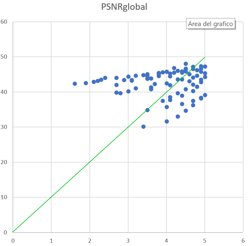
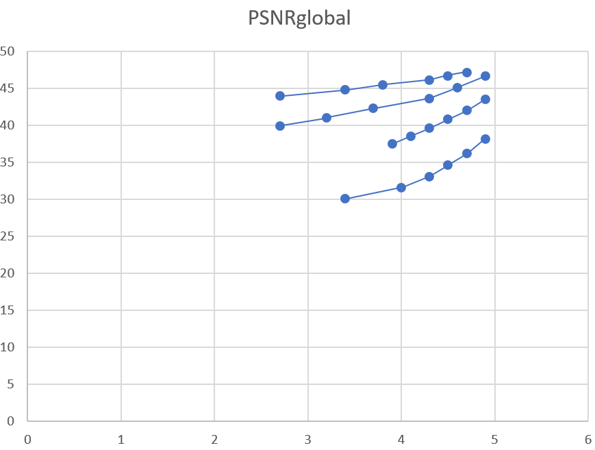
The project has required a massive campaign of subjective quality assessment performed on screens of various size. More than 14.000 quality rates related to human perception have been analyzed, enriched and used to train an ensemble of ML-algorithms. A variable set of elementary metrics (from 4 to 12) are used in different point of the project to characterize sources, encoded videos and codecs’ performance and form the vector of input features for the predictors.

The first working version of this system is going to be used by an important broadcaster in Europe and the results are very promising. For example, thanks to the training with perceptual ratings collected selectively on TVs/Tablets/Smartphones, the average bitrate of a typical TV series like Game Of Thrones with a target MOS of ~4.2 (good in a 1-5 scale) is just 350Kbps on smartphone, 900Kbps on Tablets and 2.1Mbps on TVs, down -64%, -50% and -30% respectively from the bitrates of the previous static profile.


Conclusions


ML is really a precious ally when developing optimizations in a wide range of scenarios. Previously I used to use empirical approximations that worked well but in a sub-optimal way. Now ML allows a better fitting even if it may require a considerable amount of data to work properly.

The next steps are to increase the accuracy and performance of the pipeline, but I’m also exploring the use of ML on the player side of the equation, to optimize even more also ABR heuristics and player’s logic.