H265 – part I : Technical Overview

HEVC is among us. On January 25, 2013, the ITU announced the completion of the first stage approval of the H.265 video codec standard and in the last 1 year several vendors/entities have started to work on the first implementations of H.265 encoders and decoders. Theoretically HEVC is said to be from 30 to 50% more efficient than H.264 (especially at higher resolutions) but is it really that simple ? is H.264 so close to retirement ? This is what we will try to find. First of all let’s start with a technical analysis of H.265 compared to AVC and then, in the next blog post, we will take a look at the current level of performance that is realistic to obtain in today’s H.265 encoders.

H.265/HEVC – Technical Overview

This part assumes you are sufficiently familiar with the coding techniques implemented in H.264/AVC (if you need to refresh your memory I suggest those posts: H.264 Part I, Part II).  HEVC re-uses many of the concept defined in H.264. Both are block based video encoding techniques so have the same roots and the same approach to encoding:

1. subdivision of picture in macroblocks, eventually sub-divided in blocks
2. reduction of spatial redundancy using intra-frame compression techniques
3. reduction of temporal redundancy using inter-frame compression techniques (motion estimation and compensation)
4. residual data compression using transformation & quantization
5. reduction of final redundancy in residuals and motion vectors transmission and signaling using entropy coding

HEVC can be seen as a strong evolution of AVC with some very important key features, a number of less important improvements and some simplifications.

Picture partitioning

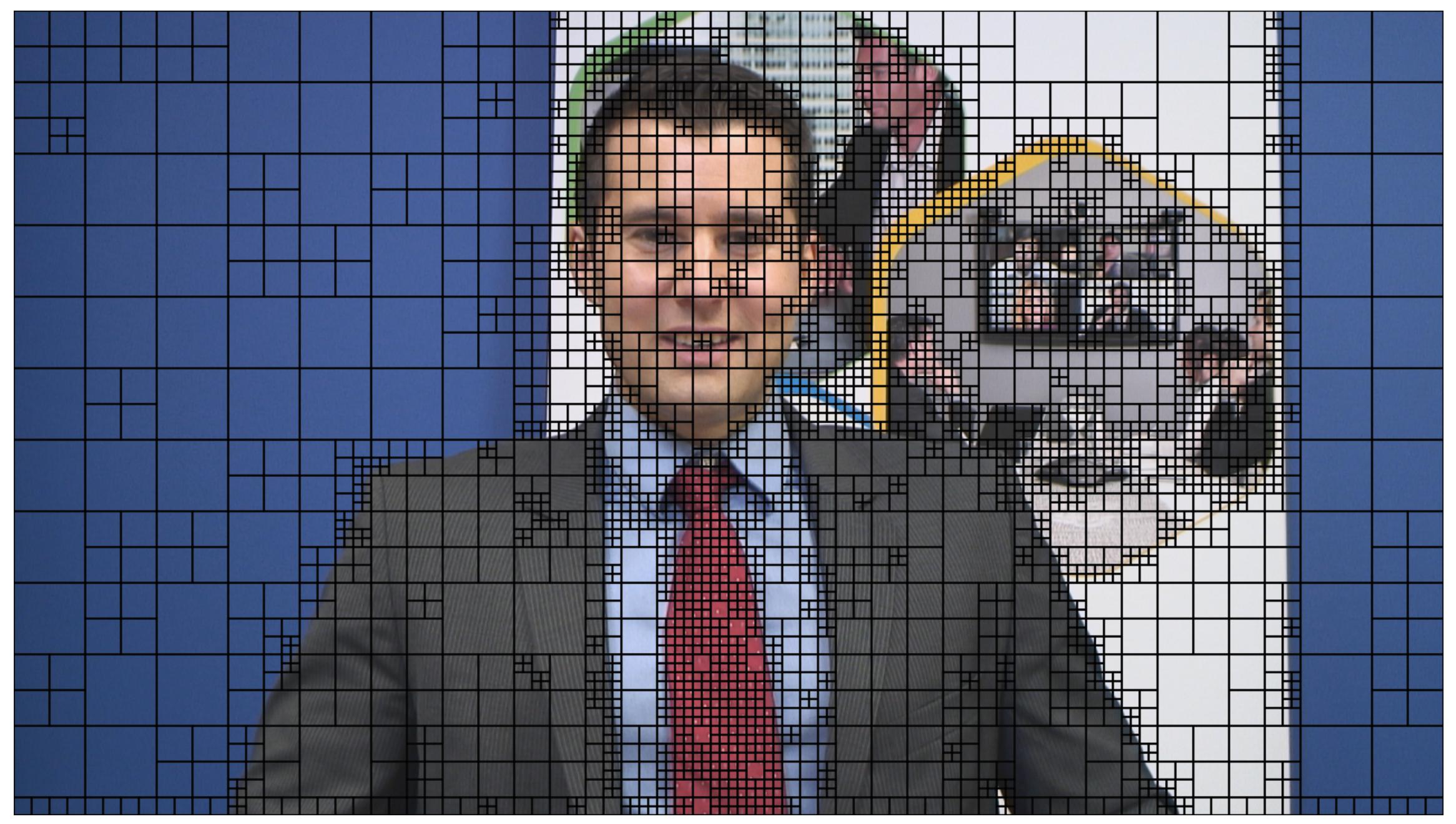
Instead of 16×16 macroblocks like in AVC, HEVC divides pictures into “coding tree blocks” (CTBs). Depending on an encoding setting the size of the CTB can be of 64×64 or limited to 32×32 or 16×16. Several studies have shown that bigger CTBs provide higher efficiency (but also higher encoding time). Each CTB can be split recursively, in a quad-tree structure, in 32×32, 16×16 down to 8×8 sub-regions, called coding units (CUs). See the picture below for an example of partitioning of a 64×64 CTB (numbers report the scan order). Each picture is furtherly partitioned in special groups of CTBs called Slices and Tiles (see also Parallel processing)

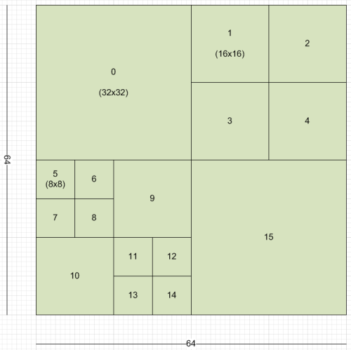
CUs are the basic unit of prediction in HEVC. Usually smaller CUs are used around detailed areas (edges and so on), while bigger CUs are used to predict flat areas.

Transform size

Each CU can be recursively split in Transform Units (TUs) with the same quad-tree approach used in CTBs. Differently from AVC that used mainly a 4×4 transform and occasionally an 8×8 transform, HEVC has several transform sizes: 32×32, 16×16, 8×8 and 4×4. From a mathematical point of view, bigger TUs are able to encode better stationary signals while smaller TUs are better at encoding smaller “impulsive” signals. The transforms are based on DCT (Discrete Cosine Transform) but the transform used for intra 4×4 is based on DST instead (Discrete Sine Transform) because several tests have evidenced a small improvement in compression. Transformation is performed with higher accuracy compared to H.264. The adaptive nature of CBT, CU and TU partitions plus the higher accuracy plus the larger transform size are among the most important features of HEVC and the reason for the performance improvement compared to AVC. HEVC implements a sophisticated scan order and coefficient signaling scheme that improves signaling efficiency. Note that unlike H.264 there’s no Hadamard nor 2×2 chroma (min chroma transform size is 4×4). HEVC drops also the support for  MBAFF or similar techniques to code interlaced video. Interlaced video can still be compressed but there’s no separation between fields and frames (only frames).

Prediction Units

We have introduced the new transform sizes just after the picture partitioning to exploit the analogy between CU and TU trees, but before transform and quantization there’s the prediction phase (inter or intra).
A CU can be predicted using one of eight partition modes (see picture below).

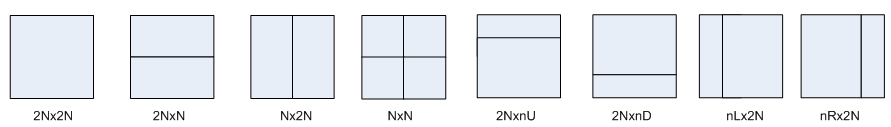
Even if a CU contains one, two or four prediction units (PUs), it can be predicted using exclusively inter-frame or intra-frame prediction technique, furthermore Intra-coded CUs can use only the square partitions 2Nx2N or NxN. Inter-coded CUs can use both square and asymmetric partitions. A number of other limitations are applied to simplify signaling. For example, no 4×4 prediction is allowed in inter-prediction and 4×8 and 8×4 are allowed only in forward prediction (so not in b-frames). Tendentially inter-prediction stops at 8×8 level.

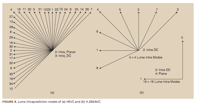
Intra prediction

HEVC has 35 different intra-prediction modes (9 in AVC). DC mode, Planar Mode and 33 directional modes. Like in AVC, intra prediction tries to recover information from surrounding blocks and works particularly well for flat areas. Intra prediction follows the TUs partition tree and so prediction modes are applied to 4×4, 8×8, 16×16 and 32×32 TUs.

Inter prediction

For motion vector prediction HEVC has two reference lists: L0 and L1. They can hold 16 references each, but the maximum total number of unique pictures is 8. Multiple instances of the same ref frame can be stored with different weights. HEVC motion estimation is much more complex than in AVC. It uses list indexing. There are two main prediction modes: Merge and Advanced MV. Each PU can use one of those methods and can have forward (a MV) or bi-directional prediction (2 MV). In Advanced MV mode a list of candidates MV is created (spatial and temporal candidates picked with a complex, probabilistic logic), when the list is created only the best candidate index is transmitted in the bitstream plus the MV delta (the difference between the real MV and the prediction). On the other side, the decoder will build and update continuously the same candidate list using the exact same rules used by the encoder and will pick-up the MV to use as estimator using the index sent by the encoder in the bitstream.
The merge mode is similar, the main difference is that the candidates’ list is calculated from neighboring MV and is not added to a delta MV. It is the equivalent of “skip” mode in AVC.

Similarly to AVC, HEVC specifies motion vectors in 1/4-pel, but uses an 8-tap filter for luma and a 4-tap 1/8-pel filter for chroma. This is considerably better than 6-tap used for luma and 2-tap (bilinear) for chroma used in AVC. An increased sub-pixel filtering accuracy improves efficiency of estimation and picture “stability” but requires much more memory accesses and so processing power (with higher battery consumption) this is why H.265 doesn’t include an inter-estimation on 4×4 regions, limits 4×8 and 8×4 estimation to be uni-directional (forward prediction) and limit to 8×8 for bi-directional. HEVC supports weighted prediction for both uni- and bi-directional PUs (always implicit weights).

HEVC uses up to 16bit per MV so at quart-pel accuracy this means a −8192 to 8191.75 rang (for luma) compared to −2048 to 2047.75 horizontally and −512 to 511.75 vertically in AVC (increased motion compensation accuracy fo 4K 8K resolutions).

Deblocking

Unlike h264 where deblocking was performed on 4×4 blocks, in HEVC deblocking is performed on the 8×8 grid only. This allows for parallel processing of deblocking (there’s no filter overlapping).  All vertical edges in the picture are deblocked first, followed by all horizontal edges. The filter is similar to AVC.

SAO

After deblocking, there’s a second optional filter. This filter is called Sample Adaptive Offset, or SAO. Similarly to deblocking filter, it is applied in the prediction loop and the result stored in the reference frames list. The objective of the filter is to fix mispredictions, encoding drift and banding on wide areas subdividing the colors in “bands” and applying an adaptive offset to them.

Entropy coding

In HEVC there’s only CABAC for entropy coding. CABAC in HEVC is almost identical to CABAC in AVC with minor changes and simplifications to allow a parallel decoding.

Parallel Processing

Since HEVC decoding is much more complex than AVC, several techniques to allow a parallel decoding have been implemented. The most important are: Tiles and Wavefront.
The picture is divided into a rectangular grid of CTBs (Tiles). Motion vector prediction and intra-prediction is not performed across tile boundaries.
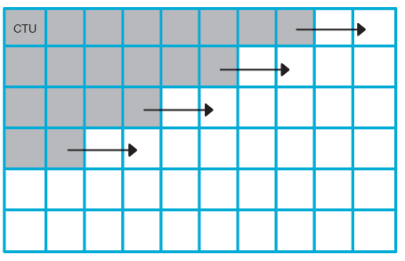
With Wavefront Each CTB row can be encoded & decoded by its own thread. Multiple rows encoding / decoding are synchronized (entropy coding state) guaranteeing that each “wavefront” CTB is surrounded by specific CTB during encoding and decoding (see picture).

Conclusion

The adaptive subdivision of picture in prediction areas, the use of advanced intra-prediction, inter-prediction and bigger transform sizes can absolutely guarantee, in the long term, a considerably higher efficiency of HEVC compared to AVC. But the complexity of the encoding is really much higher. For example, consider that in AVC a macroblock of 16×16 could have only 2 possible sub-partitions: 16 4×4 sub-blocks, or 4 8×8 sub-blocks. Now the number of possible sub-splitting of a 64×64 CTU is exceptionally higher (65536). In AVC was simple to test what of the two configurations was better for compression, but now ? New techniques must be implemented to efficiently explore the quad-tree and avoid to test every configuration out of the possible 65536.
Like AVC before, HEVC is a big optimization challenge, but the potentialities are enormous. In the next blog post we will take a look at the state of the art in H.265 encoding in mid-2014  at the beginning of 2015.